Claims reserving
riskpy.reserving is the P&C reserving toolkit: run-off triangles, the chain
ladder and its Mack standard errors, Bornhuetter–Ferguson and Cape Cod, and a
bootstrap that gives you a whole distribution of the reserve rather than a
point and a standard error.
Everything is checked against the one triangle every reserving package
agrees on — the GenIns / Taylor–Ashe triangle — and reproduces R's
ChainLadder to the unit: total reserve 18,680,856, Mack total standard
error 2,447,095.
Triangles
from riskpy import reserving

tri = reserving.Triangle([
    [357_848, 1_124_788, 1_735_330, 2_218_270],
    [352_118, 1_236_139, 2_170_033],
    [290_507, 1_292_306],
    [310_608],
], origin=[2020, 2021, 2022, 2023])

tri = reserving.Triangle.from_incremental(rows)     # if you have increments
tri = reserving.genins()                            # the reference triangle
A ragged list of lists is the natural way to type one in; a rectangular array
with NaN below the diagonal is what you get from a spreadsheet. Both work.
tri.cumulative          # (n_origin, n_dev) with NaN for the future
tri.incremental
tri.latest_diagonal
tri.link_ratios()       # individual age-to-age factors — the diagnostic view
print(tri)              # prints neatly, blanks for NaN
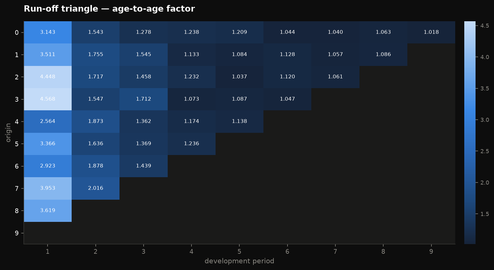
The heatmap of link ratios is the chart to look at first. The chain ladder assumes each column's factor is the same for every origin; this is where you see whether that is true.
Chain ladder
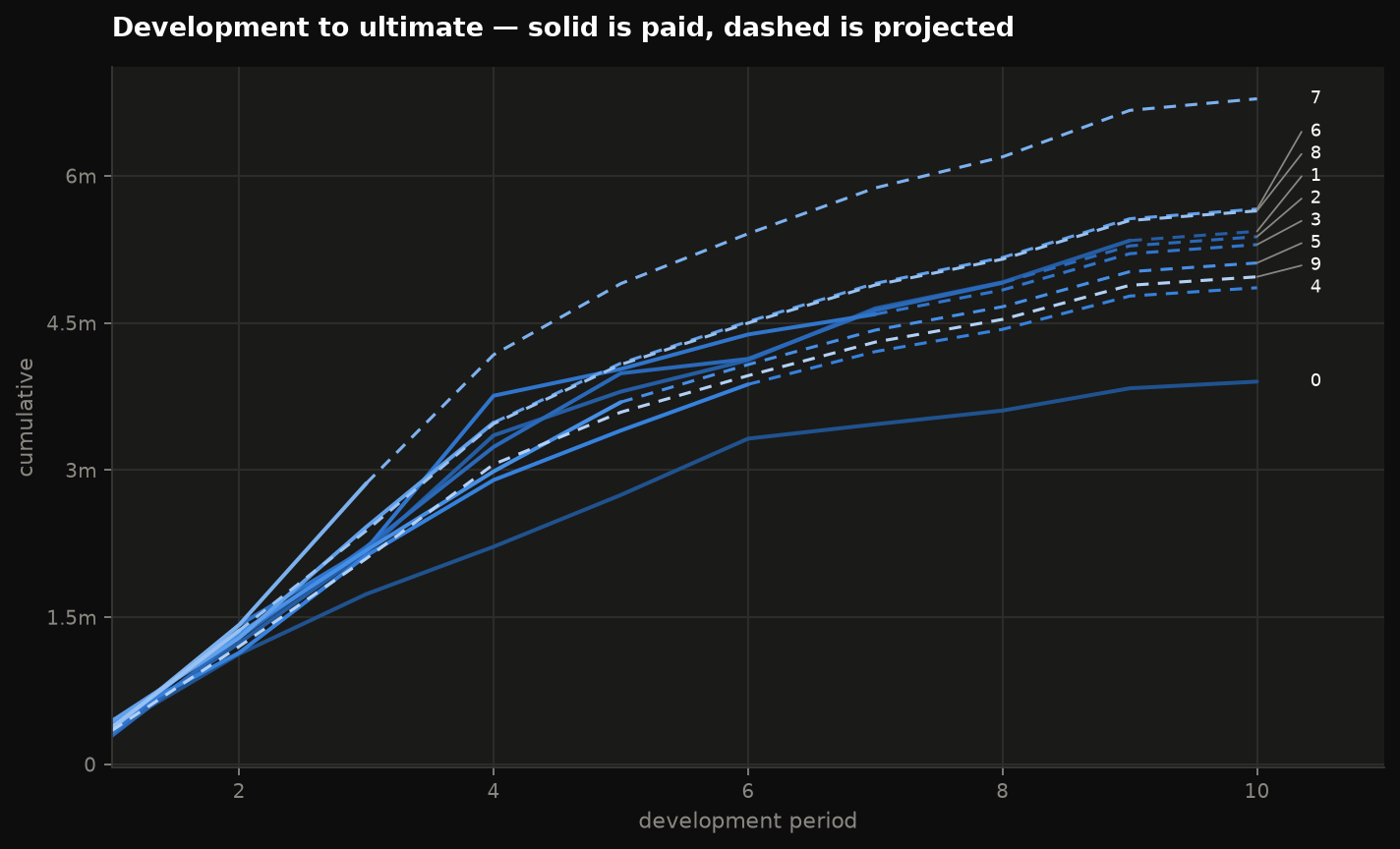
Chain ladder (volume) — 10 origins, tail 1.0000
origin      latest      cdf  developed    ultimate     reserve
0        3,901,463   1.0000     100.0%   3,901,463           0
1        5,339,085   1.0177      98.3%   5,433,719      94,634
…
9          344,014  14.4466       6.9%   4,969,825   4,625,811
--------------------------------------------------------------
total   34,358,090   1.5437      64.8%  53,038,946  18,680,856
factors  3.4906  1.7473  1.4574  1.1739  1.1038  1.0863  1.0539  1.0766  1.0177
average is "volume" (the standard weighted average), "simple" (mean of
link ratios) or "regression"; n_periods uses only the most recent
diagonals when estimating each factor. cl.factors, cl.cdf, cl.ultimate,
cl.reserve and cl.full_triangle are arrays; cl.to_frame() is a pandas
DataFrame if pandas is around.
Tail
reserving.fit_tail(cl.factors, method="exponential")    # 1.0295 on GenIns
cl = reserving.chain_ladder(tri, tail=reserving.fit_tail(cl.factors))
Regresses ln(f_k − 1) on k and extrapolates; "inverse_power" is the
alternative. A tail is a judgement, and this is a defensible starting point
for it, not a substitute.
Mack
The same chain ladder, with the standard error of every reserve — Mack's (1993) distribution-free formula, process and parameter error separately.
mk = reserving.mack_chain_ladder(tri)
mk.se, mk.process_se, mk.parameter_se     # per origin
mk.total_se                               # 2,447,095 on GenIns
mk.cv                                     # se / reserve
mk.reserve_percentile(0.995)              # 25,919,050 — lognormal matched to (reserve, se)
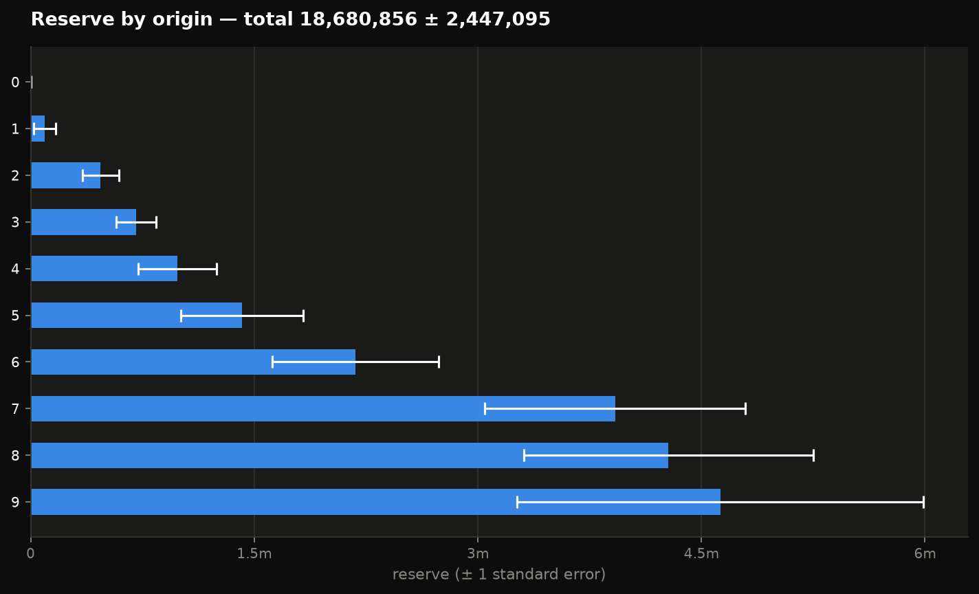
reserve_percentile assumes a lognormal shape matched to the mean and
standard error. That is the conventional choice and it is an assumption; the
bootstrap below makes none.
Expected-loss-ratio methods
When the latest diagonal is too thin to trust — young origins, a new line — the chain ladder multiplies a small number by a large factor. Bornhuetter– Ferguson blends in a prior expectation instead:
bf = reserving.bornhuetter_ferguson(tri, premiums=premiums, expected_loss_ratio=0.60)
cc = reserving.cape_cod(tri, premiums=premiums)      # estimates the loss ratio from the data
ec = reserving.expected_claims(tri, ultimates_prior=prior_ultimates)
Cape Cod (Stanard–Bühlmann) sets the expected loss ratio to
Σ latest / Σ (premium × % developed), so the whole triangle votes on it;
cc.extra["expected_loss_ratio"] tells you what it chose. Each returns a
ReserveResult with the same summary(), ultimate, reserve and
total_reserve as the chain ladder.
The relationship between them is an identity, and it is in the verification suite: Bornhuetter–Ferguson with the prior set to the chain-ladder ultimate is the chain ladder.
Bootstrap
England & Verrall's (2002) over-dispersed Poisson bootstrap: back-fit the incremental triangle, resample the scaled Pearson residuals, refit, project, and add process error — a few thousand times.
bs = reserving.bootstrap_chain_ladder(tri, n=2000, seed=1)
print(bs.summary())
bs.percentile(0.995)          # 28,235,828
bs.reserves                   # (n, n_origin) — every simulated reserve
Bootstrap chain ladder (ODP, process=odp) — 2,000 samples, seed 1, phi 52,601.36
origin      latest  CL reserve        mean         se     cv       75.0%       95.0%       99.5%
…
total   34,358,090  18,680,856  18,785,639  3,054,568  0.163  20,673,658  23,930,411  28,235,828
bs.result() wraps the simulated totals as a
riskpy.mc.Result, so every chart and every risk measure
in the rest of the library applies to a reserve distribution unchanged:
from riskpy import viz

total = bs.result()
total.var(0.995), total.tvar(0.995)
viz.distribution(total)
viz.exceedance(total)
process is "odp" (gamma-approximated process error with the fitted scale),
"gamma", or "none" for parameter uncertainty alone.
Agreement with the compiled core
The C++ LossTriangle has done volume-weighted chain ladder since 0.2. The
Python chain_ladder reproduces its ultimates to 1e-6 relative on every
triangle in the test suite, and the verification suite checks it on GenIns
each run. The Python side is where the uncertainty methods live; the C++ side
is the one to call from a tight loop.
References
- Mack, T. (1993). Distribution-free calculation of the standard error of chain ladder reserve estimates. ASTIN Bulletin, 23(2).
- England, P. & Verrall, R. (2002). Stochastic claims reserving in general insurance. British Actuarial Journal, 8(3).
- Bornhuetter, R. & Ferguson, R. (1972). The actuary and IBNR. PCAS, 59.
- Taylor, G. & Ashe, F. (1983) — the triangle.