RiskPY
A risk and actuarial engine with a C++ core and a Python modelling layer you can read. The compiled part — factor rating, loss triangles, Fourier aggregate loss, exposure and experience rating — has no Python dependencies at all. The modelling layers on top cover most of what a risk or actuarial team reaches for in a week, and every identity they claim is checked by a verification suite that runs on every push.
pip install open-riskpy          # core, zero dependencies
pip install "open-riskpy[sim]"   # + NumPy: simulation and the numeric layers
pip install "open-riskpy[viz]"   # + Matplotlib: the charts
The idea in nine lines
A Monte Carlo simulation is what you reach for when the formula is too big to solve. Rather than integrating, you feed the formula random inputs a few hundred thousand times and look at the distribution that comes out.
from riskpy.mc import Model, Poisson, LogNormal, Normal

model = Model(
    claim_count = Poisson(mean=140),
    severity    = LogNormal.from_moments(mean=18_000, sd=42_000),
    inflation   = Normal(mean=0.043, sd=0.012),
)
model.correlate("claim_count", "inflation", 0.3)     # dependence, if you have a view

@model.formula
def annual_loss(claim_count, severity, inflation):
    return claim_count * severity * (1 + inflation)

result = model.run(200_000, seed=42, sampling="lhs")
print(result.summary())
result.plot("dashboard")
Your formula is called once, with arrays — two hundred thousand trials is
a single vectorised expression, not a Python loop. sampling="lhs" draws a
Latin hypercube, which cuts the noise on the mean by a large factor for free.
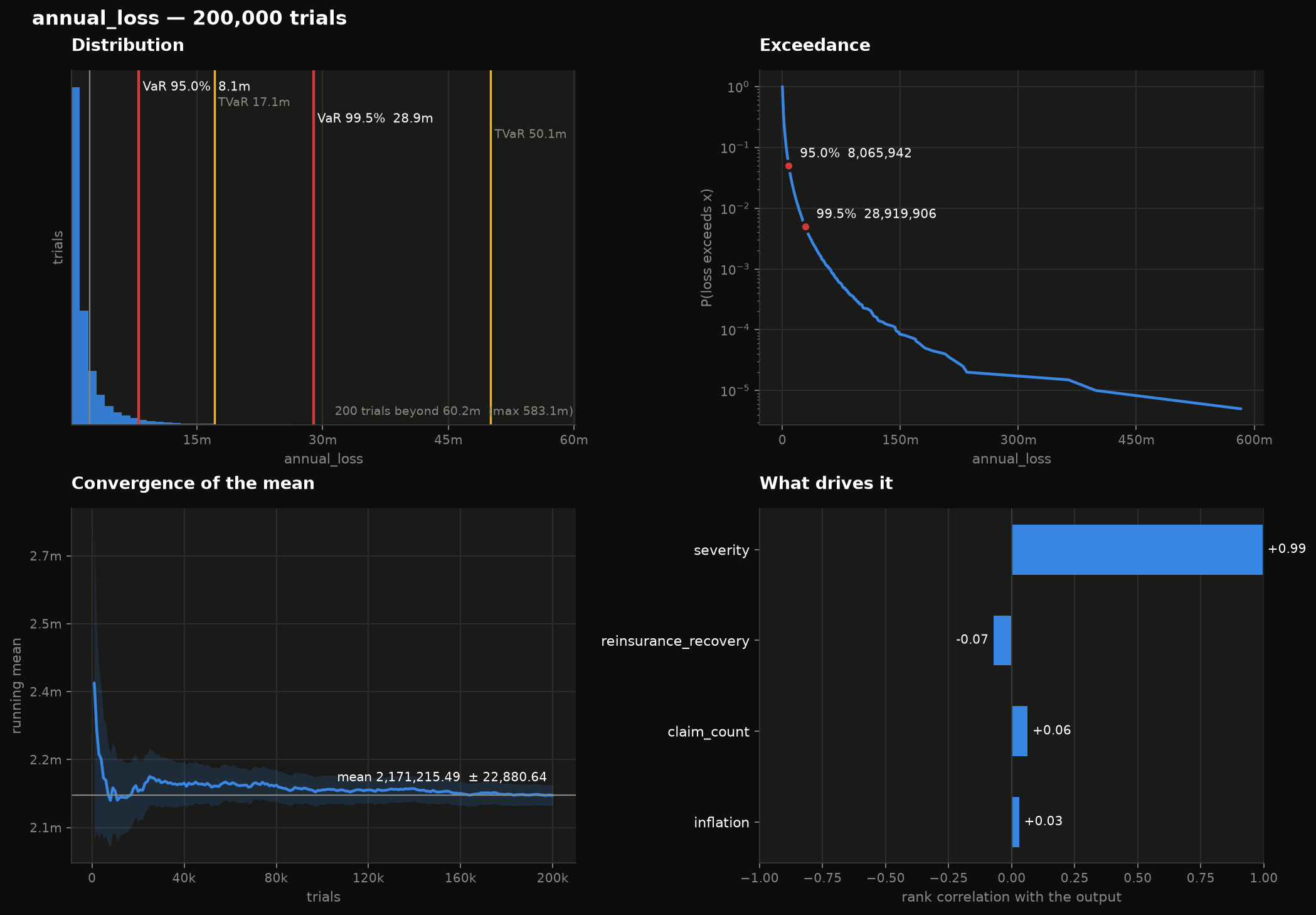
Then ask it things
result.var(0.995)          # Value at Risk at 99.5%
result.tvar(0.995)         # and the mean loss beyond it
result.prob_above(5e6)     # P(annual loss > 5m)
result.sensitivity()       # which input is driving the answer
result.standard_error      # did I run enough trials?
result.describe()          # the lot, as a dict
What is in the box
-
Twenty distributions with a full analytic layer (
pdf,cdf,ppf,moments), mixtures and truncation, Latin hypercube sampling, rank correlation by Iman–Conover, and a copula hook. -
Twenty-two charts, one theme, light and dark, both palettes validated for contrast and colour-vision deficiency. Every chart returns a
Figureand none callsshow(). -
Black–Scholes with Greeks and implied vol in pure Python; GBM and jump-diffusion paths; historical, parametric and expected-shortfall VaR; Heston by Fourier inversion.
-
Life tables (Gompertz, Makeham, the AMLCR standard table), every insurance and annuity present value, premiums, reserves, joint lives — pure Python, reproducing the textbook to its printed precision.
-
Chain ladder, Mack standard errors, Bornhuetter–Ferguson, Cape Cod, and an ODP bootstrap. Reproduces R's
ChainLadderon GenIns to the unit. -
Yield curves (bootstrap, Nelson–Siegel, Svensson), bonds with duration, convexity, DV01 and z-spread, and Vasicek and CIR with closed-form bonds and simulated paths.
-
Merton, hazard rates and CDS, the Vasicek / Basel ASRF model with IRB capital, a one-factor copula portfolio simulation, rating transitions.
-
Every identity the library claims — put–call parity,
A_x = 1 − d·ä_x, Mack's standard error on GenIns, the Basel risk-weight table — checked on every push and published here.
Four charts that answer four questions
-
Where is the tail?
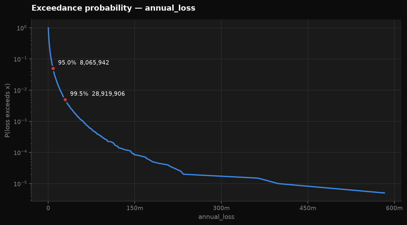
viz.exceedance(result)— P(loss > x), log scale, with VaR called out. -
Did I run enough trials?
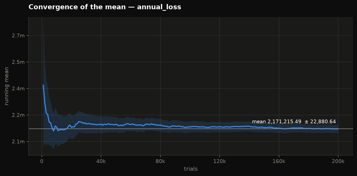
viz.convergence(result)— running mean with a 95% band. Still narrowing at the right edge means no. -
What is driving it?
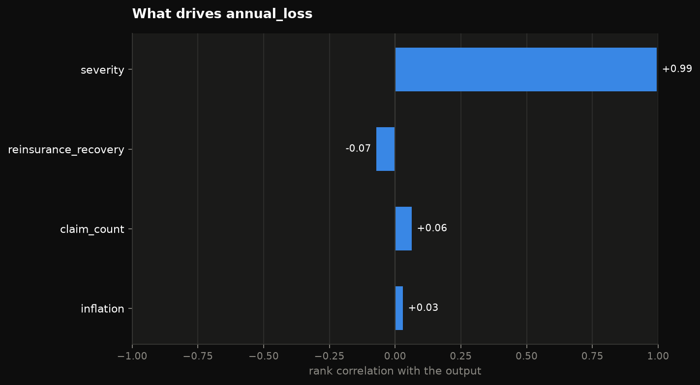
viz.tornado(result)— rank correlation of each input with the output. -
How do scenarios compare?
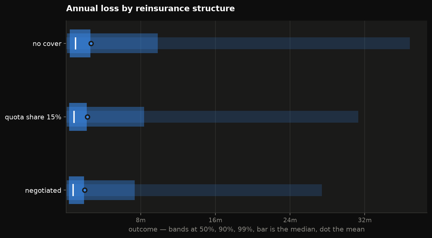
viz.spread({...})— quantile ranges per scenario, readable for dozens.
The compiled core
Everything below is C++ behind a Python interface and needs nothing installed beyond the wheel:
from riskpy import FactorModel, LossTriangle, FourierTransform, MonteCarloSimulator

model = FactorModel(initial_base_rate=1000.0)
model.add_multiplier("state", "FL", 3.0)
model.add_numeric_band_multiplier("age", 16, 25, 2.0)
model.calculate({"state": "FL", "age": 19.0})            # 6000.0

# Severity always 1 → aggregate is Poisson(λ), with no sampling error at all
pmf = FourierTransform.compound_poisson_pmf([0.0, 1.0], expected_frequency=2.0, grid_size=64)

sim = MonteCarloSimulator(trials=200_000, seed=7)
losses = sim.simulate_aggregate_loss(5.0, 8.0, 0.5)
See How it works, Architecture and the API reference for the core.
Where to go next
- Monte Carlo — the full distribution list and the
ResultAPI - Visualisation — every chart, and the rules they follow
- Verification — what is checked, and the latest report