Interest rates¶

riskpy.rates covers the term structure: discounting conventions, yield curves, bonds and their sensitivities, and the two classic short-rate models.

Bond and curve arithmetic is pure Python; the path simulators need NumPy.

pip install open-riskpy          # curves, bonds, closed-form bond prices
pip install "open-riskpy[sim]"   # + Vasicek and CIR paths

Conventions¶

Rates are annualised decimals. compounding is "continuous", "annual", or an integer m for m times a year. Mixing them is the mistake everyone makes once, so the conversion is explicit:

from riskpy import rates

rates.discount_factor(0.05, t=2.0)                    # e^{-0.10}
rates.discount_factor(0.05, t=2.0, compounding=2)     # (1 + 0.05/2)^{-4}
rates.zero_rate(df, t, compounding)
rates.convert_rate(0.05, "annual", "continuous")      # ln 1.05
rates.forward_rate(df_1, t_1, df_2, t_2)

Yield curves¶

curve = rates.YieldCurve(times=[1, 2, 5, 10, 30],
                         zero_rates=[0.020, 0.025, 0.030, 0.033, 0.035])

curve.zero(7.0)               # interpolated zero rate
curve.df(7.0)                 # discount factor
curve.forward(2.0, 5.0)       # the 3-year rate, 2 years forward
curve.instantaneous_forward(7.0)
curve.par_rate(10.0, frequency=2)
curve.shift(25)               # parallel, in basis points
curve.points()                # (times, zeros, forwards) — for viz.curve

interpolation="linear" is linear in the zero rate — the market default, with small jumps in the forward curve at the knots. "log_linear" is linear in the log discount factor, which is a piecewise-constant forward curve. Extrapolation is flat in both, and the docstring says so because a 30-year curve asked for a 40-year discount factor answers confidently.

Building one¶

rates.YieldCurve.flat(0.03)
rates.YieldCurve.from_discount_factors(times, dfs)
rates.YieldCurve.bootstrap(par_rates=[0.020, 0.025, 0.028, 0.030, 0.031],
                           maturities=[1, 2, 3, 4, 5], frequency=1)
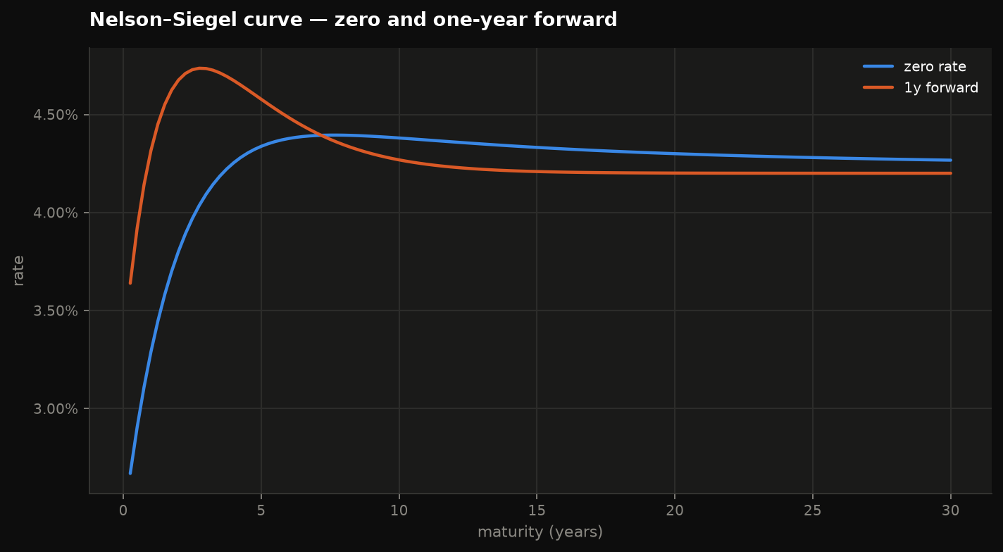
rates.YieldCurve.nelson_siegel(beta0=0.042, beta1=-0.018, beta2=0.028, tau=2.0)
rates.YieldCurve.svensson(beta0, beta1, beta2, beta3, tau1, tau2)

The bootstrap reproduces its input par rates to 1e-10 — that is the round-trip test. The parametric curves keep their formula and evaluate it at any maturity, so the limits hold exactly: zero(0) = β₀ + β₁ and zero(∞) = β₀.

Yield curve

Bonds¶

bond = rates.Bond(face=100, coupon=0.05, maturity=10, frequency=2)

bond.price(ytm=0.04)              # 108.1757
bond.yield_to_maturity(108.0)     # 4.0205%
bond.macaulay_duration(0.04)      # 8.0809 years
bond.modified_duration(0.04)      # 7.9225
bond.convexity(0.04)              # 75.47
bond.dv01(0.04)                   # 0.0857 per basis point
bond.cashflows()                  # [(0.5, 2.5), (1.0, 2.5), …, (10.0, 102.5)]

bond.price_from_curve(curve)
bond.z_spread(price, curve)       # the parallel shift that reprices it

duration_price_change(price, modified_duration, convexity, dy) is the second-order approximation, and the tests check that it beats the first-order one for a 100 bp move rather than assuming so.

Identities in the suite: a bond priced at its coupon rate is worth par at any frequency; a zero's Macaulay duration is its maturity; modified is Macaulay over 1 + y/m; DV01 matches a bumped price; ytm(price(y)) = y.

Short-rate models¶

rates.vasicek_zero_bond(r=0.03, t=0, T=5, kappa=0.5, theta=0.04, sigma=0.02)  # 0.835450
rates.cir_zero_bond(r=0.03, t=0, T=5, kappa=0.5, theta=0.04, sigma=0.05)      # 0.834237

rates.vasicek_curve(r0, kappa, theta, sigma)      # a YieldCurve from the model
rates.cir_curve(r0, kappa, theta, sigma)

paths = rates.vasicek_paths(r0, kappa, theta, sigma, T=5, steps=250, trials=20_000, seed=1)
paths = rates.cir_paths(r0, kappa, theta, sigma, T=5, steps=250, trials=20_000, seed=1)

Vasicek paths use the exact Gaussian transition, not an Euler step, so there is no discretisation error in the simulated rates — only in the integral you take of them. CIR uses full-truncation Euler and warns when the Feller condition 2κθ > σ² fails, because then the simulation misbehaves even though the closed-form price is fine.

Both closed forms are checked against Monte Carlo averages of exp(−∫r dt) — Vasicek in the verification suite, CIR in the tests — and both collapse to the deterministic exp(−∫r dt) as σ → 0. That second check is more delicate than it sounds: the CIR formula has a 1/σ² exponent, and the textbook arrangement loses every digit below about σ = 10⁻⁶. The implementation uses a log1p form that does not.

θ is risk-neutral

The long-run mean in both bond formulas is the risk-neutral one. A θ estimated from historical rates needs the market price of risk added before it prices anything, and the difference is the term premium. The Vasicek yield curve also does not converge to θ at long maturities but to θ − σ²/(2κ²) — a surprise the first time.

References¶

Hull, J. Options, Futures, and Other Derivatives, ch. 4 and 31.
Vasicek, O. (1977). An equilibrium characterization of the term structure.
Cox, Ingersoll & Ross (1985). A theory of the term structure of interest rates.
Nelson, C. & Siegel, A. (1987). Parsimonious modeling of yield curves.