Quant finance
riskpy.quant is three layers, separated by what they cost you to install.
| Layer | Needs | What is in it |
|---|---|---|
| Closed form | nothing | black_scholes, greeks, implied_vol |
| Simulation | NumPy | gbm_paths, merton_jump_paths |
| Portfolio risk | NumPy | historical_var, parametric_var, expected_shortfall |
| Transform pricing | NumPy | heston_price |
The closed-form functions are pure Python, so they work in the same lean install as the C++ core:
pip install open-riskpy        # black_scholes, greeks, implied_vol
pip install "open-riskpy[sim]" # + paths, VaR, Heston
Conventions throughout: T is in years, rates and volatilities are
annualised decimals (0.05, not 5), and q is the continuous dividend yield.
Black–Scholes
from riskpy import quant

quant.black_scholes(S=100, K=100, T=1.0, r=0.05, sigma=0.2)
# 10.450583572
quant.black_scholes(S=100, K=100, T=1.0, r=0.05, sigma=0.2, kind="put")
# 5.573526022
The degenerate cases are handled rather than left to divide by zero: at expiry, or at zero volatility, you get the discounted intrinsic value.
Greeks
Units are the ones people quote, not the raw derivatives: vega is per one
percentage point of volatility, theta is per calendar day, rho is per
percentage point of rate. Multiply vega and rho by 100, and theta by 365, if you
want the mathematical partials.
Each Greek is tested against a numerical derivative of the price, which catches whole classes of sign error that a single reference value would not.
Implied volatility
Bisection, not Newton. Newton is faster when it works, but vega collapses for deep in- and out-of-the-money options and it diverges exactly where you most want an answer. Two hundred bisection steps is still instant.
A price outside the no-arbitrage bounds raises ValueError rather than
returning something — which is the useful answer, because it means the quote is
stale or wrong, not that the solver gave up.
Paths
paths = quant.gbm_paths(S0=100, mu=0.07, sigma=0.22, T=1.0,
                        steps=252, trials=20_000, seed=42)
paths.shape          # (20000, 253)
Uses the exact log-Euler solution rather than an Euler approximation of the SDE. GBM has a closed-form transition density, so there is no discretisation error to accept and no reason to accept one.
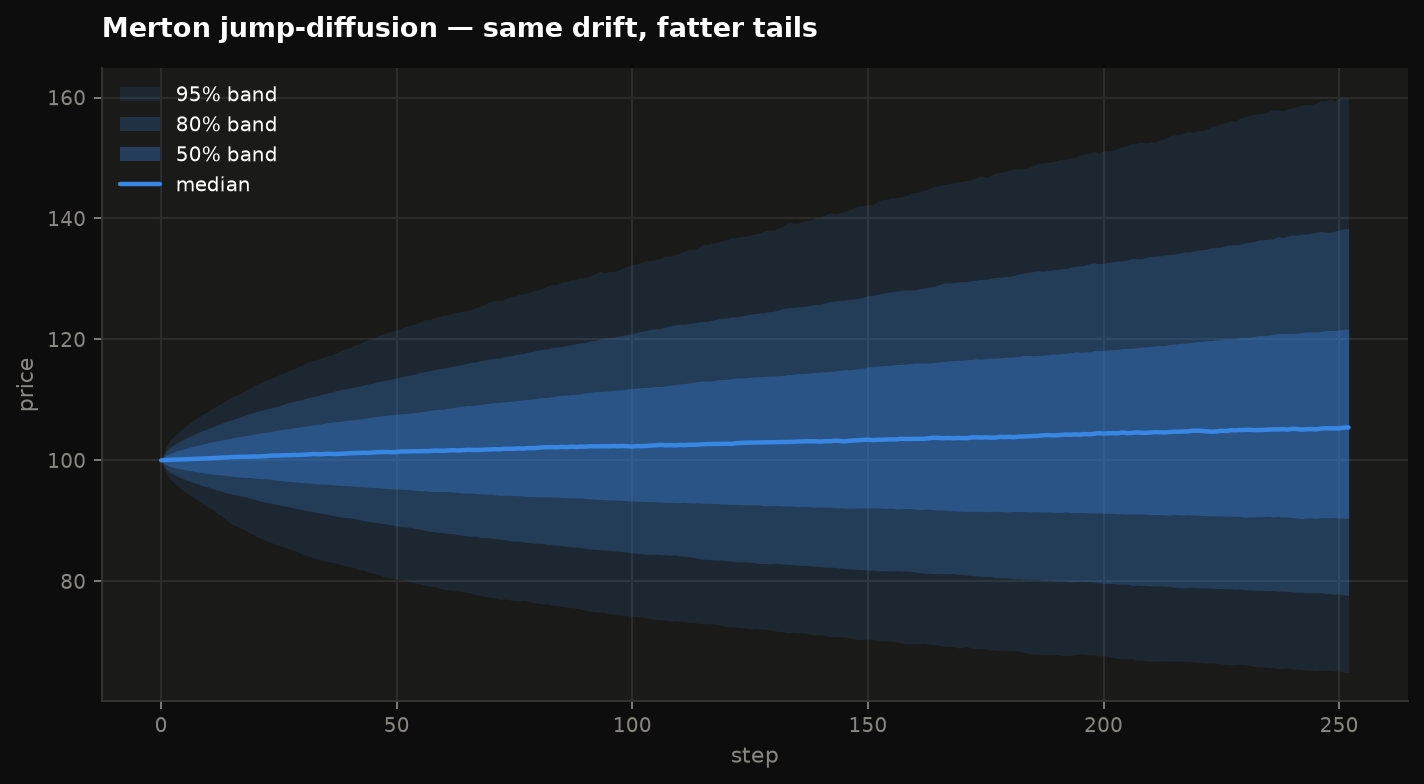
jumps = quant.merton_jump_paths(
    S0=100, mu=0.07, sigma=0.18, T=1.0,
    jump_intensity=1.2, jump_mean=-0.05, jump_sd=0.12,
    trials=20_000, seed=42,
)
The drift carries the usual compensator, so the process keeps expected return
mu — without it the jumps quietly add drift and nothing prices sensibly.
Feed either straight to viz.fan.
Portfolio risk
quant.historical_var(returns, level=0.99)      # empirical, positive loss
quant.parametric_var(returns, level=0.99)      # normal assumption
quant.expected_shortfall(returns, level=0.99)  # mean loss beyond VaR
All three return a positive number for a loss.
historical_var makes no distributional assumption, which is its strength and
its limit: it can never report a loss worse than the worst one in your sample.
parametric_var understates tail risk whenever returns are fat-tailed, which is
nearly always. Compare the two rather than trusting either alone — a large gap
between them is itself the finding.
parametric_var also accepts moments directly:
Heston, by Fourier inversion
This is the concrete answer to "the formula is too big".
Heston has no closed-form option price. It does have a closed-form characteristic function — so rather than simulating a million paths, you integrate the transform once. Faster, and exact to the quadrature error.
quant.heston_price(
    S=100, K=100, T=1.0, r=0.03,
    v0=0.04,        # initial variance
    kappa=2.0,      # mean-reversion speed
    theta=0.04,     # long-run variance
    xi=0.5,         # vol of vol
    rho=-0.7,       # spot/vol correlation, negative for equities
)
It uses the "little Heston trap" formulation, which keeps the complex logarithm on its principal branch. The textbook form is algebraically identical and numerically wrong past a couple of years — a real trap, hence the name.
The Feller condition
If 2·kappa·theta <= xi**2, variance can reach zero and you get a
RuntimeWarning. The price is still computable and real calibrations
violate the condition routinely, so it warns rather than refuses — but a
simulation of those same parameters will behave badly.
The sanity check worth knowing: as xi → 0 with v0 = theta, variance becomes
deterministic and Heston must reproduce Black–Scholes at sigma = sqrt(theta).
That identity is in the test suite, and it is what catches a sign error in the
characteristic function.
quant.black_scholes(S=100, K=100, T=1, r=0.03, sigma=0.2)
quant.heston_price(S=100, K=100, T=1, r=0.03,
                   v0=0.04, kappa=2.0, theta=0.04, xi=1e-6, rho=0.0)
# agree to ~1e-3
upper and nodes control the integration range and resolution. Raise nodes
for very short maturities, where the integrand oscillates fastest.
Relationship to the C++ core
The compiled FourierTransform class does the same trick for aggregate loss
distributions — compound Poisson severity via FFT — and is the faster path when
you need the whole distribution rather than one price. Same idea, different
problem: a transform you can write down beats a simulation you have to wait for.