Monte Carlo¶

riskpy.mc is for the case where the formula is too awkward to solve. Instead of integrating, you feed it random inputs a few hundred thousand times and read the distribution that falls out.

pip install "open-riskpy[sim]"

The shape of it¶

from riskpy import viz
from riskpy.mc import (
    Model, Poisson, LogNormal, Normal, PERT,
    Gamma, NegativeBinomial, Pareto, Mixture, Truncated, Categorical,
)

model = Model(
    claim_count          = Poisson(mean=140),
    severity             = LogNormal.from_moments(mean=18_000, sd=42_000),
    inflation            = Normal(mean=0.043, sd=0.012),
    reinsurance_recovery = PERT(low=0.0, mode=0.15, high=0.45),
)

@model.formula
def annual_loss(claim_count, severity, inflation, reinsurance_recovery):
    gross = claim_count * severity * (1 + inflation)
    return gross * (1 - reinsurance_recovery)

result = model.run(200_000, seed=42)

Your formula is called once, with NumPy arrays of length trials — not once per trial. Two hundred thousand trials is a single vectorised expression.

If your formula has branching NumPy cannot express, pass vectorised=False and it is looped instead. Correct, just slower.

Always pass a seed

seed=42 makes a run reproducible. Without one you get a different answer every time, which is fine for exploring and miserable for a report someone else has to check.

Without the decorator¶

simulate() is the same engine with no Model object, which reads better when you are sweeping scenarios in a loop:

from riskpy.mc import simulate, Constant

result = simulate(
    lambda claims, severity: claims * severity,
    trials=100_000, seed=42, label="annual loss",
    claims=Poisson(mean=140),
    severity=LogNormal.from_moments(mean=18_000, sd=42_000),
)

Or let the model sweep for you — same seed for every scenario, so the differences are the scenarios and not the noise:

scenarios = model.sweep("reinsurance_recovery", {
    "no cover":        Constant(0.0),
    "quota share 15%": Constant(0.15),
    "negotiated":      PERT(0.05, 0.25, 0.5),
}, trials=100_000, seed=42)
viz.compare(scenarios)

Distributions¶

Continuous	Discrete	Composite
`Normal(mean, sd)`	`Poisson(mean)`	`Constant(value)`
`LogNormal(mu, sigma)`	`NegativeBinomial(n_success, p)`	`Empirical(data)`
`Uniform(low, high)`	`Bernoulli(p)`	`Categorical(values, probs)`
`Triangular(low, mode, high)`	`Binomial(trials, p)`	`Mixture([dists], weights)`
`PERT(low, mode, high, lam=4)`		`Truncated(dist, low, high)`
`Exponential(scale)`
`Gamma(shape, scale)`
`Beta(a, b)`
`Pareto(xm, alpha)`
`Weibull(shape, scale)`
`StudentT(df, loc, scale)`

Alternative constructors exist where the raw parameters are never the numbers you actually have:

LogNormal.from_moments(mean=18_000, sd=42_000)     # not mu and sigma of the log
LogNormal.from_median_cv(median=12_000, cv=1.8)    # how reinsurance quotes them
Gamma.from_moments(mean=12, sd=4)
NegativeBinomial.from_mean_dispersion(mean=140, dispersion=2.4)

Pareto with a light tail index

Pareto has an infinite mean for alpha <= 1 and infinite variance for alpha <= 2. The sample mean will still print a number. It will not mean anything — and Pareto(...).moments() will say inf, which is the honest answer.

Parameters are validated when the distribution is constructed, not when it is sampled — a negative standard deviation is a typo, and finding out after a ten-second run is worse than useless.

The analytic layer¶

Every distribution knows more than how to sample itself:

d = Gamma(2.5, 1.7)
d.pdf(x), d.cdf(x), d.ppf(q)     # vectorised; scalar in, scalar out
d.moments()                       # Moments(mean=4.25, variance=7.225) with .sd and .cv
d.support()                       # (0.0, inf)

The quantile functions are accurate to around 1e-10 relative or better across the whole range, and to machine precision in the extreme tails, where the survival function is inverted directly rather than the CDF. They are what make Latin hypercube sampling, truncation and correlated inputs possible, and they are built on a dependency-free special-function layer (incomplete gamma and beta, Student-t) that is checked against SciPy in the test suite without ever requiring it.

Composites¶

Mixture([LogNormal(8, 1), Pareto(50_000, 2.5)], weights=[0.9, 0.1])   # attritional + large
Truncated(LogNormal(8, 1), high=1_000_000)                            # a policy limit
Truncated(Normal(0.04, 0.02), low=0.0)                                # a rate that cannot go negative
Categorical([0.9, 1.0, 1.15], probs=[0.2, 0.6, 0.2])                  # scenario weights

Truncated samples by inversion, so it never rejects and never loops, and its moments are integrated numerically to about 1e-8 relative.

Dependence¶

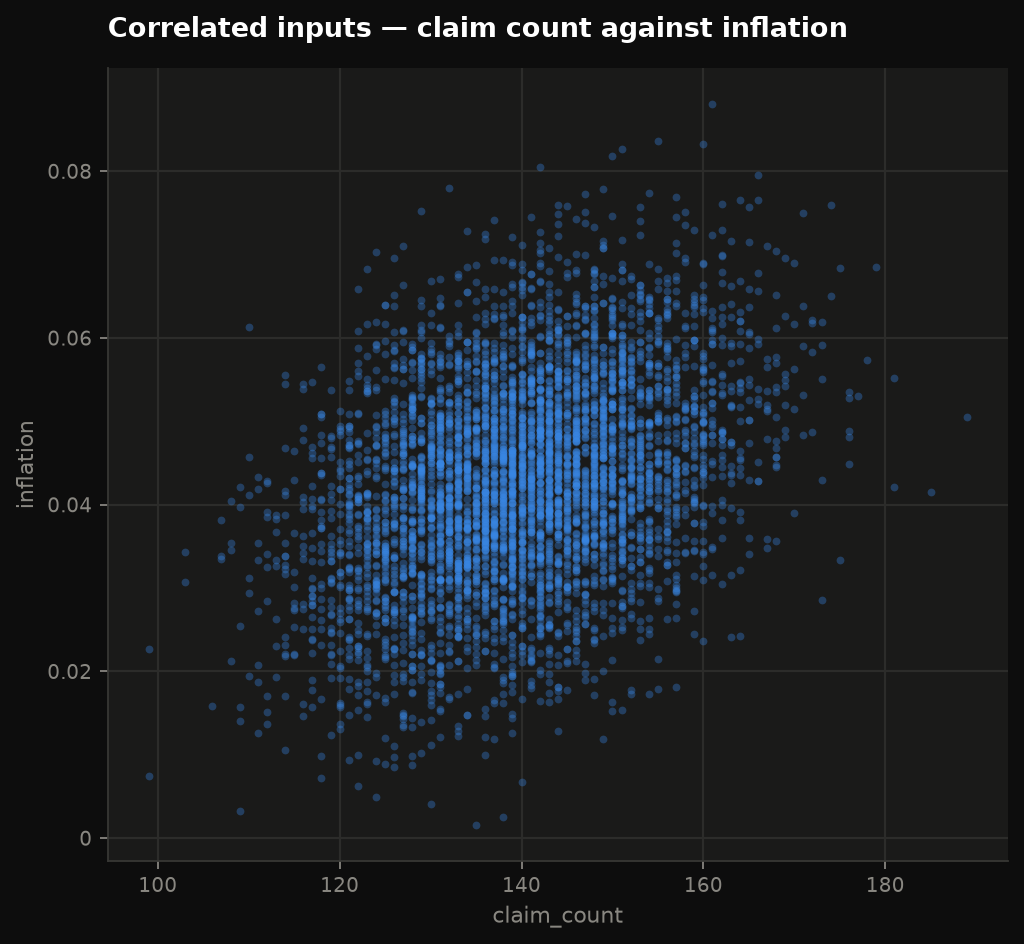
Inputs are independent unless you say otherwise. Two ways to say otherwise:

model.correlate("claim_count", "inflation", 0.3)     # Spearman rank correlation
model.correlate("severity", "inflation", 0.2)

result = simulate(fn, ..., correlation={("a", "b"): 0.7})   # or a full matrix

This is Iman–Conover: the samples are drawn independently and then re-paired so their ranks follow a correlated normal score matrix. The marginals are untouched — every sampled value is kept — which is why it works with any distribution and with Latin hypercube draws. The recovered rank correlation lands within 0.01 of the target at 100k trials.

A set of pairwise correlations can be jointly impossible; the error names the smallest eigenvalue rather than letting a Cholesky failure surface later.

For tail dependence a correlation cannot express, simulate accepts copula= — any object with .dim and .uniforms(n, rng) returning an (n, dim) array of correlated uniforms, which are then pushed through each distribution's ppf.

Scatter

Latin hypercube sampling¶

result = model.run(200_000, seed=42, sampling="lhs")

One draw from each of n equal-probability strata, in random order. Same marginal, far less noise: the standard deviation of the estimated mean falls by a factor of two to three for typical loss models, at no cost. Distributions without a quantile function fall back to plain sampling for that input.

Reading the result¶

result.mean, result.std, result.median
result.skewness, result.kurtosis    # how badly a normal approximation will do
result.standard_error               # how much the mean would move on a new seed
result.percentile(99.5)
result.var(0.995)                   # Value at Risk
result.tvar(0.995)                  # mean loss beyond VaR
result.cdf(5e6)                     # P(output <= x)
result.prob_above(5e6)
result.describe()                   # a dict of the lot
result.values                       # the raw array

summary() returns the headline table as a string. For the model on this page, with its two correlations and sampling="lhs":

Monte Carlo — annual_loss
  trials       200,000   seed 42
  mean         2,178,785.66   ± 23,229.21 (95% CI)
  std dev      5,300,213.95   skew +25.06
  min / max    1,809.39 / 737,951,531.59

  level        VaR              TVaR
  50.000%          847,483.26     3,988,906.14
  75.000%        2,134,575.78     6,608,175.09
  90.000%        4,916,632.64    11,708,574.21
  95.000%        8,128,962.41    17,180,392.03
  99.000%       20,664,267.01    37,318,456.01
  99.500%       29,220,862.23    50,413,329.25

Quantile queries sort once and cache the order, so asking for a dozen VaR levels costs one sort, not twelve.

VaR and TVaR¶

var(0.995) is the loss exceeded 0.5% of the time. tvar(0.995) is the average of those worst 0.5% of outcomes, so it is always at least as large.

Prefer TVaR for the reason regulators do: VaR tells you where the threshold is and nothing whatsoever about how bad things get past it. Two portfolios with identical VaR can have wildly different tails.

Did I run enough trials?¶

standard_error is how much the mean would wobble on a different seed. It shrinks with the square root of the trial count, so ten times the precision costs a hundred times the work — or one switch to sampling="lhs".

n, running_mean, half_width = result.convergence()
result.plot("convergence")

What is driving the answer?¶

for name, correlation in result.sensitivity():
    print(f"{name:24} {correlation:+.2f}")

severity                 +0.99
inflation                +0.23
reinsurance_recovery     -0.07
claim_count              +0.06

Spearman rank correlation by default — the relationship between an input and a total is usually monotonic and rarely linear. method="pearson" for the linear case and method="contribution" for each input's share of explained variance. Plot it with result.plot("tornado").

Exporting¶

result.to_frame()      # pandas DataFrame (needs pandas): every input column plus the output
result.histogram(60)   # (edges, counts)
result.exceedance_curve()

Common errors, and what they mean¶

"The formula returned shape (), expected (200000,)" — your formula collapsed the arrays to a scalar. Usually an if (use np.where), a min() (use np.minimum), or a sum() that should not be there.

"12,431 of 200,000 trials produced NaN or infinity" — nearly always a division by a variable that can reach zero, or a log of one that can go negative. The count tells you how much of the tail is involved.

"claim_count must be a Distribution, got float" — wrap fixed numbers in Constant(...). This is deliberate: silently accepting a bare number makes it easy to freeze an input you meant to vary.

"correlation matrix is not positive semi-definite" — the pairwise correlations you asked for cannot all hold at once. Reduce the strongest ones.